Shortest Path Algorithms
Given a weighted graph $G = (V, E)$ with a weight function $w: E \to \mathbb{R}$, the shortest path problem asks: what is the minimum total weight path from one vertex to another (or to all other vertices)? The weight of a path is the sum of the weights of its edges. We study three major algorithms, each suited to different situations depending on whether weights can be negative, and whether we want one source or all pairs.
Think of this as planning a road trip. Each road (edge) has a travel cost (weight), like distance, time, or toll. We want to find the cheapest route from our starting city to a destination, or sometimes to every other city at once.
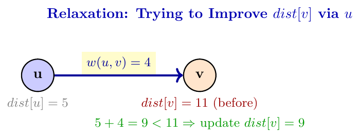
All shortest path algorithms are built around a single basic operation called relaxation. For an edge $(u,v)$ with weight $w(u,v)$, relaxing this edge means: "Can we improve our current best known distance to $v$ by going through $u$?" \[ \text{if } dist[u] + w(u,v) < dist[v]: \quad dist[v] \gets dist[u] + w(u,v), \quad parent[v] \gets u \] Every algorithm in this chapter (Dijkstra, Bellman-Ford, Floyd-Warshall) is just a different strategy for deciding which edges to relax, and in what order.
Single-Source: Dijkstra's Algorithm
Dijkstra's algorithm finds the shortest path from a single source vertex $s$ to every other vertex in the graph, but it requires all edge weights to be non-negative. The core strategy is greedy: at every step, we pick the unvisited vertex with the smallest known distance, mark it as finalized, and relax all of its outgoing edges.
Think of it like water spreading outward from a source, but unlike BFS (which spreads in equal steps), Dijkstra always expands to the "nearest" unexplored point first, where "nearest" accounts for edge weights.
Imagine you are standing in a city, and you want to find the cheapest taxi fare to every other location. You always first finalize the fare to whichever place is currently cheapest to reach (among places not yet finalized), because once a place is the cheapest remaining option, there is no way a longer, more expensive route could ever beat it (since all fares are non-negative, going through a costlier intermediate stop can never reduce the total cost).
At each step, Dijkstra picks the unvisited vertex $u$ with minimum tentative distance $dist[u]$, and declares this distance final. This is correct only because all weights are non-negative. If $u$ has the smallest tentative distance among all unvisited vertices, then any other path to $u$ through a vertex that is not yet finalized would have to pass through an edge with non-negative weight, making that alternate path's length at least as long as $dist[u]$ already is. So no shorter path to $u$ can possibly be discovered later.
Algorithm: Dijkstra(G, w, s)
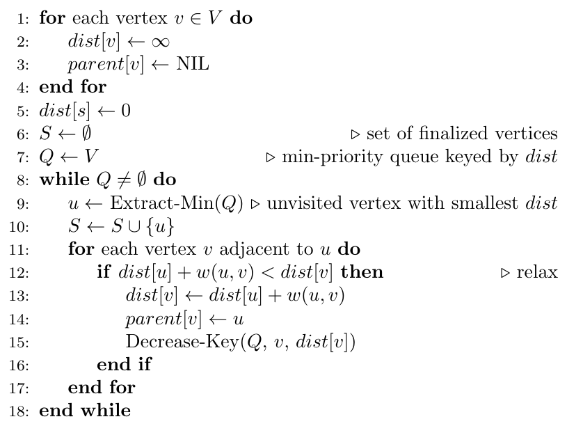
The running time depends entirely on how the priority queue is implemented:
Simple array: Finding the minimum each time takes $O(V)$ (linear scan), done $V$ times, giving $O(V^2)$ for Extract-Min calls. Each edge relaxation is $O(1)$, giving $O(E)$ total for relaxations. Total: $O(V^2 + E) = O(V^2)$ (since $E \le V^2$).
Binary min-heap: Extract-Min takes $O(\log V)$, done $V$ times: $O(V \log V)$. Decrease-Key takes $O(\log V)$, done at most $O(E)$ times: $O(E \log V)$. Total: $O((V+E) \log V)$.
Fibonacci heap (advanced): Extract-Min is $O(\log V)$ amortized, Decrease-Key is $O(1)$ amortized, giving $O(E + V \log V)$, the best known bound.
For dense graphs ($E \approx V^2$), the simple array is actually competitive or better. For sparse graphs ($E \approx V$), the heap-based version is much faster.
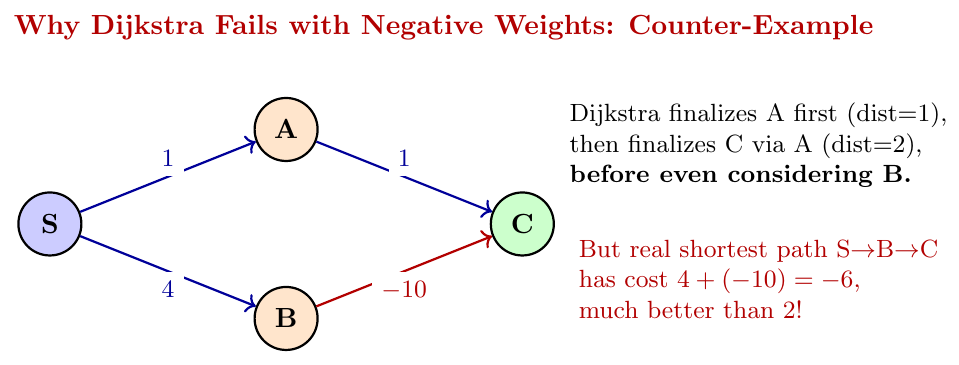
Dijkstra's greedy strategy relies on the assumption that once a vertex is finalized (marked visited with its minimum distance locked in), no future relaxation can ever improve it. This assumption breaks if negative edge weights exist, because a path through a vertex we haven't visited yet (which currently looks "farther") could later take a very negative edge and become shorter overall than what we already finalized.
Dijkstra: Step-by-Step Trace (Standard Example)
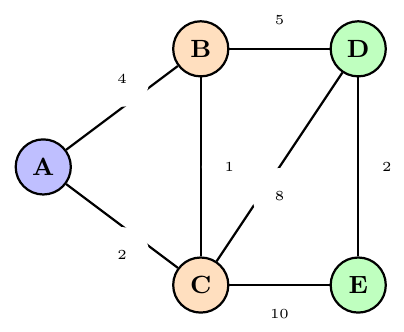
Graph: vertices $\{A, B, C, D, E\}$, edges with weights: $A{-}B{:}4$, $A{-}C{:}2$, $B{-}C{:}1$, $B{-}D{:}5$, $C{-}D{:}8$, $C{-}E{:}10$, $D{-}E{:}2$.
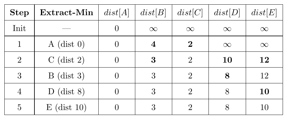
Explanation of each step:
Step 1: Extract A (dist 0). Relax $A\to B$: $0+4=4 < \infty$, set $dist[B]=4$. Relax $A\to C$: $0+2=2<\infty$, set $dist[C]=2$.
Step 2: Smallest unvisited is C (dist 2). Relax $C\to B$: $2+1=3 < 4$, improve $dist[B]=3$. Relax $C\to D$: $2+8=10$, set $dist[D]=10$. Relax $C\to E$: $2+10=12$, set $dist[E]=12$.
Step 3: Smallest unvisited is B (dist 3). Relax $B\to D$: $3+5=8 < 10$, improve $dist[D]=8$.
Step 4: Smallest unvisited is D (dist 8). Relax $D\to E$: $8+2=10 < 12$, improve $dist[E]=10$.
Step 5: Smallest unvisited is E (dist 10). No outgoing edges to relax further.
Final shortest distances from A: $B=3, C=2, D=8, E=10$.
Dijkstra: Complex Trace (Directed Graph with Reordering)
Directed graph: $S\to A(10)$, $S\to B(5)$, $B\to A(3)$, $B\to D(2)$, $A\to C(1)$, $D\to A(7)$, $D\to C(9)$, $C\to D(4)$. This graph tests whether the relaxation order causes re-evaluation.
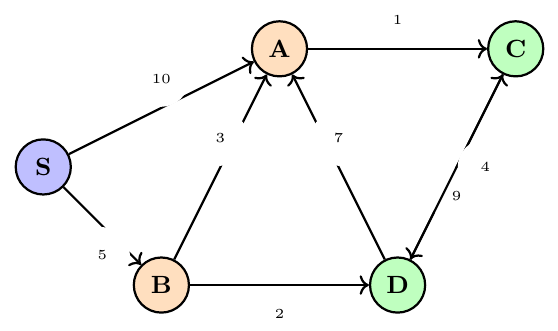
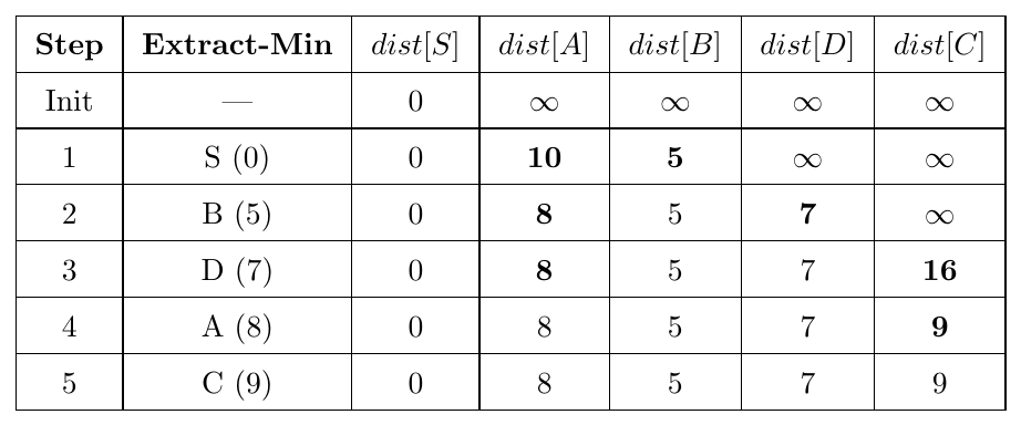
Key observation: Notice that $dist[A]$ was first set to 10 (via $S\to A$), then improved to 8 (via $S\to B\to A$), demonstrating that a vertex's tentative distance can be relaxed multiple times before it is finally extracted. Once A is extracted (finalized) at distance 8, it will never change again, this is the core greedy guarantee.
Assumption: All edge weights must be non-negative. This is non-negotiable; the algorithm's correctness proof depends on it.
Property: Once a vertex is extracted from the priority queue (finalized), its distance value is guaranteed optimal and never changes again.
Property: Dijkstra works for both directed and undirected graphs, as long as weights are non-negative.
Advantage: Much faster than Bellman-Ford for non-negative weights, especially with a good priority queue: $O((V+E)\log V)$ vs $O(VE)$.
Advantage: Naturally produces a shortest-path tree (via the parent pointers), giving paths to every reachable vertex from the source in one run.
Limitation: Cannot handle negative edge weights at all, even without negative cycles; it can give incorrect (too large) results.
Limitation: Does not directly extend to all-pairs shortest paths; running it from every vertex gives $O(V(V+E)\log V)$, which is often worse than Floyd-Warshall for dense graphs.
import heapq

def dijkstra(graph, n, source):
    """
    graph: dict of u -> list of (v, weight)
    Returns dist[] and parent[] arrays.
    """
    dist   = [float('inf')] * n
    parent = [-1] * n
    dist[source] = 0

    pq = [(0, source)]          # (distance, vertex)
    visited = [False] * n

    while pq:
        d, u = heapq.heappop(pq)
        if visited[u]:
            continue             # stale entry, skip
        visited[u] = True

        for v, w in graph[u]:
            if not visited[v] and dist[u] + w < dist[v]:
                dist[v]   = dist[u] + w
                parent[v] = u
                heapq.heappush(pq, (dist[v], v))

    return dist, parent


# --- Driver Code ---
# Graph: S=0, A=1, B=2, D=3, C=4
graph = {
    0: [(1, 10), (2, 5)],
    1: [(4, 1)],
    2: [(1, 3), (3, 2)],
    3: [(1, 7), (4, 9)],
    4: [(3, 4)],
}

dist, parent = dijkstra(graph, 5, 0)
print("Distances from S:", dist)     # [0, 8, 5, 7, 9]
print("Parents:", parent)
Single-Source: Bellman-Ford Algorithm
Bellman-Ford also finds shortest paths from a single source, but unlike Dijkstra, it works even when edge weights are negative (as long as there is no negative weight cycle reachable from the source). Instead of greedily picking the closest vertex, Bellman-Ford takes a simpler, more brute-force approach: relax every single edge, and repeat this entire process $V-1$ times.
A shortest path between any two vertices in a graph with $V$ vertices can have at most $V-1$ edges (since a simple path visits at most $V$ vertices, hence at most $V-1$ edges; a path with a cycle is never shorter than the same path with the cycle removed, as long as there's no negative cycle).
Each full pass over all edges guarantees that the shortest path using at most $k$ edges is correctly computed after the $k$-th pass. So after $V-1$ passes, we are guaranteed to have found the shortest path using at most $V-1$ edges, which covers every possible simple shortest path in the graph.
Algorithm: Bellman-Ford(G, w, s)
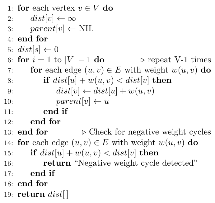
After the $V-1$ main iterations, we do one more pass over all edges. If any edge can still be relaxed (i.e., $dist[u] + w(u,v) < dist[v]$), this means the shortest path estimate is still improving beyond what $V-1$ edges should allow. This can only happen if there is a negative weight cycle reachable from the source, since such a cycle allows us to keep looping around it, making the "shortest path" infinitely small (undefined).
Bellman-Ford: Step-by-Step Trace
Directed graph: $S\to A(6)$, $S\to C(7)$, $A\to C(8)$, $A\to D(5)$, $A\to B(-4)$, $C\to D(-3)$, $C\to E(9)$, $D\to B(-1)$, $B\to D(7)$ wait — let's use the classic CLRS example: $S\to T(6), S\to Y(7), T\to X(5), T\to Y(8), T\to Z(-4), X\to T(-2), Y\to X(-3), Y\to Z(9), Z\to X(7), Z\to S(2)$.
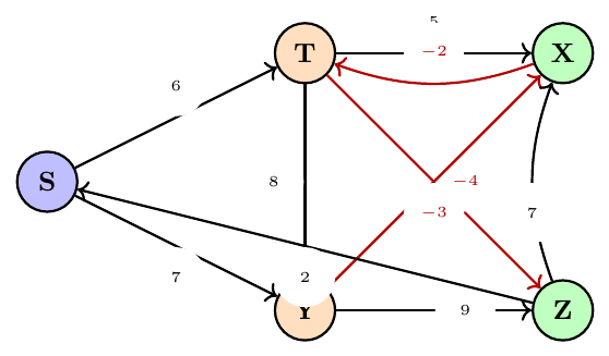
Processing order of edges: $(S,T), (S,Y), (T,X), (T,Y), (T,Z), (X,T), (Y,X), (Y,Z), (Z,X), (Z,S)$.
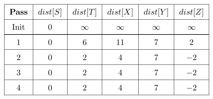
Pass 1: $(S,T)$: $0+6=6\to dist[T]=6$. $(S,Y)$: $0+7=7\to dist[Y]=7$. $(T,X)$: $6+5=11\to dist[X]=11$. $(T,Y)$: $6+8=14$, no improvement. $(T,Z)$: $6-4=2\to dist[Z]=2$. $(X,T)$: $11-2=9$, no improvement. $(Y,X)$: $7-3=4<11\to dist[X]=4$. $(Y,Z)$: $7+9=16$, no improvement. $(Z,X)$: $2+7=9$, no improvement. $(Z,S)$: $2+2=4$, no improvement.
Pass 2: $(T,Z)$: now $dist[T]=6$ still, so no change yet in this pass's early edges. Key change: $(X,T)$: $4-2=2<6\to dist[T]=2$. Later edges then use updated $dist[T]=2$: $(T,Z)$ re-examined only in pass 3 since edges are processed once per pass in fixed order, so by pass 2 end, $dist[T]=2$ propagates further in Pass 3: $(T,Z)$: $2-4=-2<2\to dist[Z]=-2$.
Pass 3, 4: No further changes; values have converged.
Final shortest distances from S: $T=2, X=4, Y=7, Z=-2$.
Verification pass (negative cycle check): Re-examine all edges once more; no edge can be relaxed further, confirming no negative weight cycle exists.
Assumption: The graph can have negative edge weights, but must not have a negative weight cycle reachable from the source (or the algorithm correctly detects this instead of producing wrong output).
Property: After $k$ passes, $dist[v]$ correctly equals the shortest path to $v$ using at most $k$ edges.
Property: The order in which edges are processed within a single pass does not affect the final correctness, though it may affect how fast convergence happens (sometimes fewer than $V-1$ passes are needed in practice).
Advantage: Handles negative weights, unlike Dijkstra.
Advantage: Can explicitly detect negative weight cycles, a very useful diagnostic capability (e.g., detecting arbitrage opportunities in currency exchange graphs).
Advantage: Simple to implement; works with just an edge list, no priority queue needed.
Limitation: Much slower than Dijkstra for the same non-negative-weight graph: $O(VE)$ vs $O((V+E)\log V)$.
Limitation: If a negative cycle is reachable from the source, the notion of "shortest path" to vertices affected by that cycle is undefined (distances can be made arbitrarily small by looping).
def bellman_ford(edges, n, source):
    """
    edges: list of (u, v, weight) tuples
    Returns dist[], parent[], and whether a negative cycle exists.
    """
    dist   = [float('inf')] * n
    parent = [-1] * n
    dist[source] = 0

    # Relax all edges V-1 times
    for _ in range(n - 1):
        updated = False
        for u, v, w in edges:
            if dist[u] != float('inf') and dist[u] + w < dist[v]:
                dist[v]   = dist[u] + w
                parent[v] = u
                updated = True
        if not updated:           # early exit: no change this pass
            break

    # One more pass: detect negative weight cycle
    has_negative_cycle = False
    for u, v, w in edges:
        if dist[u] != float('inf') and dist[u] + w < dist[v]:
            has_negative_cycle = True
            break

    return dist, parent, has_negative_cycle


# --- Driver Code ---
# S=0, T=1, X=2, Y=3, Z=4
edges = [
    (0,1,6), (0,3,7), (1,2,5), (1,3,8), (1,4,-4),
    (2,1,-2), (3,2,-3), (3,4,9), (4,2,7), (4,0,2),
]

dist, parent, neg_cycle = bellman_ford(edges, 5, 0)
print("Distances:", dist)             # [0, 2, 4, 7, -2]
print("Negative cycle?", neg_cycle)   # False
All-Pairs: Floyd-Warshall Algorithm
Floyd-Warshall solves the all-pairs shortest path problem: finding the shortest distance between every pair of vertices $(i,j)$, all at once. It uses dynamic programming, based on a simple but powerful idea: for every pair $(i,j)$, we consider whether the shortest path should pass through an intermediate vertex $k$, trying every possible $k$, one at a time.
Let $d^{(k)}[i][j]$ denote the shortest path from $i$ to $j$ using only vertices $\{1, 2, \ldots, k\}$ as intermediate vertices (the endpoints $i$ and $j$ themselves are always allowed). The recurrence is: \[ d^{(k)}[i][j] = \min\Big(d^{(k-1)}[i][j], \; d^{(k-1)}[i][k] + d^{(k-1)}[k][j]\Big) \] In words: the shortest path either does not use vertex $k$ at all (so it's the same as before), or it does pass through $k$ (so it splits into a path from $i$ to $k$, plus a path from $k$ to $j$, both using only vertices up to $k-1$). We take the smaller of these two options. The base case is $d^{(0)}[i][j] = w(i,j)$ (direct edge weight, or $\infty$ if no edge, and 0 if $i=j$).
Since each $d^{(k)}$ only depends on $d^{(k-1)}$, we can use a single 2D array and update it in-place as $k$ increases from 1 to $V$.
Algorithm: Floyd-Warshall(W)
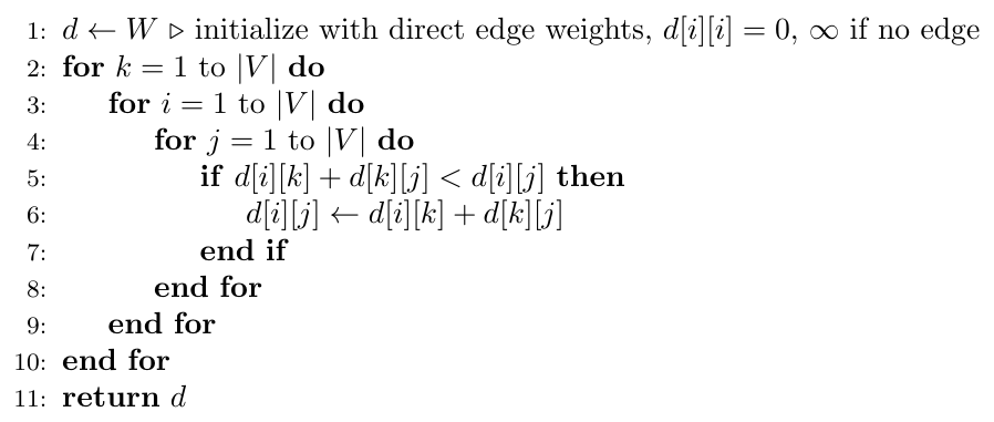
Three nested loops, each running $V$ times, gives $\Theta(V^3)$ time. We store a $V \times V$ matrix, giving $\Theta(V^2)$ space. This is efficient for dense graphs where we want all-pairs distances; running Dijkstra from every vertex would take $O(V \cdot (V+E)\log V)$, which for dense graphs ($E \approx V^2$) becomes $O(V^3 \log V)$, actually worse than Floyd-Warshall's clean $O(V^3)$.
Floyd-Warshall: Step-by-Step Matrix Trace
Vertices $\{1, 2, 3, 4\}$, directed edges: $1\to2(3), 1\to3(8), 1\to4(-4), 2\to4(1), 2\to3(7), 3\to1(2), 4\to3(-5), 4\to1(6)$. This matches the classic CLRS Floyd-Warshall example.
\[ d^{(0)} = \begin{pmatrix} 0 & 3 & 8 & -4 \\ \infty & 0 & 7 & 1 \\ 2 & \infty & 0 & \infty \\ 6 & \infty & -5 & 0 \end{pmatrix} \]
Check if any $d[i][1] + d[1][j] < d[i][j]$. For example, $d[3][2]$: direct is $\infty$, via vertex 1: $d[3][1] + d[1][2] = 2 + 3 = 5$. Update $d[3][2] = 5$. Similarly $d[3][4]$: $d[3][1]+d[1][4] = 2+(-4) = -2 < \infty$, update. \[ d^{(1)} = \begin{pmatrix} 0 & 3 & 8 & -4 \\ \infty & 0 & 7 & 1 \\ 2 & 5 & 0 & -2 \\ 6 & 9 & -5 & 0 \end{pmatrix} \] (Row 4, column 2: $d[4][1]+d[1][2] = 6+3=9 < \infty$, so updated.)
Check $d[i][2] + d[2][j]$. For instance $d[1][3]$: direct is 8, via vertex 2: $d[1][2]+d[2][3] = 3+7=10$, not better. $d[3][3]$ via 2: $5 + \infty$, no change. $d[1][4]$ via 2: $3+1=4$, not better than $-4$. No improvements occur at this step for most entries except checking carefully all combinations; the matrix stays effectively the same at this stage for this particular graph. \[ d^{(2)} = \begin{pmatrix} 0 & 3 & 8 & -4 \\ \infty & 0 & 7 & 1 \\ 2 & 5 & 0 & -2 \\ 6 & 9 & -5 & 0 \end{pmatrix} \]
Check $d[i][3] + d[3][j]$. $d[2][1]$: direct $\infty$, via 3: $d[2][3]+d[3][1] = 7+2=9$. Update $d[2][1]=9$. $d[4][2]$: via 3: $d[4][3]+d[3][2] = -5+5=0 < 9$, update $d[4][2]=0$. $d[2][4]$: via 3: $7+(-2)=5$, not better than 1. \[ d^{(3)} = \begin{pmatrix} 0 & 3 & 8 & -4 \\ 9 & 0 & 7 & 1 \\ 2 & 5 & 0 & -2 \\ 6 & 0 & -5 & 0 \end{pmatrix} \]
Check $d[i][4] + d[4][j]$. $d[1][3]$: via 4: $d[1][4]+d[4][3] = -4+(-5)=-9 < 8$. Update $d[1][3]=-9$. $d[2][1]$: via 4: $1+6=7 < 9$. Update $d[2][1]=7$. $d[2][3]$: via 4: $1+(-5)=-4 < 7$. Update $d[2][3]=-4$. $d[3][2]$: via 4: $-2+0=-2 < 5$. Update $d[3][2]=-2$. \[ d^{(4)} = \begin{pmatrix} 0 & 3 & -9 & -4 \\ 7 & 0 & -4 & 1 \\ 2 & -2 & 0 & -2 \\ 6 & 0 & -5 & 0 \end{pmatrix} \]
This is the final all-pairs shortest distance matrix. Reading row $i$, column $j$ gives the shortest distance from $i$ to $j$.
After running the algorithm to completion, check the diagonal entries $d[i][i]$. In a graph with no negative weight cycles, every $d[i][i]$ should remain 0 (the trivial zero-length path from $i$ to itself). If any $d[i][i] < 0$ after all iterations, it means there is a cycle through $i$ with negative total weight, since the "shortest path" from $i$ back to itself has become negative.
Assumption: Works correctly with negative edge weights, but like Bellman-Ford, requires no negative weight cycles for the result to be meaningful (otherwise, detect it via negative diagonal entries).
Property: The order of considering intermediate vertices $k = 1, 2, \ldots, V$ matters for correctness; we must process them in a complete, increasing sequence (any fixed full ordering works, not necessarily by vertex label).
Property: Can be used on both directed and undirected graphs (undirected simply means $w(i,j) = w(j,i)$).
Advantage: Gives all pairs shortest paths in a single clean run, with simple nested-loop code, no complex data structures.
Advantage: Can detect negative weight cycles anywhere in the graph (not just those reachable from one source, unlike Bellman-Ford which only checks from a chosen source).
Advantage: Simple to extend for computing transitive closure (reachability) by replacing min/+ with OR/AND operations.
Limitation: $O(V^3)$ time can be too slow for very large sparse graphs; running Dijkstra $V$ times (with a heap) is often faster when $E \ll V^2$.
Limitation: $O(V^2)$ space can also be prohibitive for very large $V$.
def floyd_warshall(W, n):
    """
    W: n x n matrix, W[i][j] = weight of edge i->j,
       float('inf') if no edge, 0 if i == j
    Returns the all-pairs shortest distance matrix.
    """
    d = [row[:] for row in W]   # deep copy

    for k in range(n):
        for i in range(n):
            for j in range(n):
                if d[i][k] + d[k][j] < d[i][j]:
                    d[i][j] = d[i][k] + d[k][j]

    # Check for negative weight cycles
    for i in range(n):
        if d[i][i] < 0:
            print(f"Negative weight cycle detected through vertex {i}")

    return d


# --- Driver Code ---
INF = float('inf')
# Vertices: 1,2,3,4 -> indices 0,1,2,3
W = [
    [0,   3,   8,  -4],
    [INF, 0,   7,   1],
    [2,   INF, 0,   INF],
    [6,   INF, -5,  0],
]

result = floyd_warshall(W, 4)
for row in result:
    print(row)

# Output:
# [0, 3, -9, -4]
# [7, 0, -4, 1]
# [2, -2, 0, -2]
# [6, 0, -5, 0]
Choosing the Right Algorithm
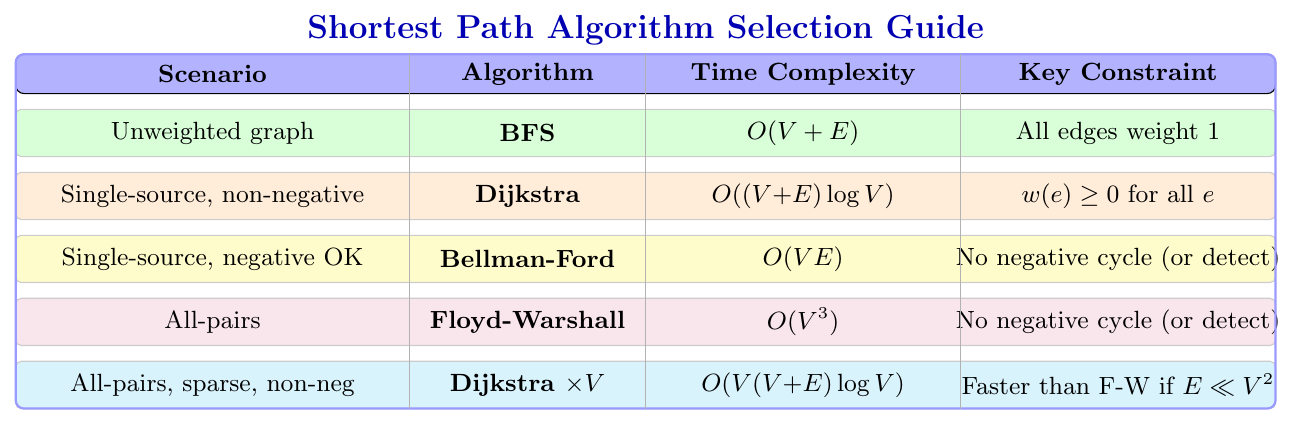
Are all weights 1 (unweighted)? Use BFS. Simplest and fastest, $O(V+E)$.
Single source needed, and are all weights non-negative? Use Dijkstra. It is the fastest correct algorithm for this case.
Single source needed, but negative weights possible? Use Bellman-Ford. Slower, but correctly handles negatives and can detect negative cycles.
Need distances between every pair of vertices? Use Floyd-Warshall if the graph is dense or $V$ is small-to-moderate. If the graph is sparse and weights are non-negative, running Dijkstra from each vertex can be faster.